Linear classifier from scratch

5 minute read

Introduction

In this project I build a linear classifier from scratch using MNIST dataset (a standard digit classification dataset). Given a 28 \(\times\) 28 image containing a digit from 0 to 9, our goal is deducing which digit the image corresponds to. The dataset has 60,000 training and 10,000 test examples. The data can be downloaded from http://yann.lecun.com/exdb/mnist/.

Formatting the data

As the data is in idx format we need convert into the format which can be read by the numpy.

X_train = idx2numpy.convert_from_file('DATA/train-images-idx3-ubyte')

Y_train = idx2numpy.convert_from_file('DATA/train-labels-idx1-ubyte')

X_test = idx2numpy.convert_from_file('DATA/t10k-images-idx3-ubyte')

Y_test = idx2numpy.convert_from_file('DATA/t10k-labels-idx1-ubyte')

We further need to format the data to obtain a 2-D dataset as each input X is of dimensions 28 \(\times\) 28 we need to convert this matrix into a vector of size 784 each. Each label y is a digit from 0 to 9 we need to apply one-hot encoding on y and convert it to a vector \(y^{oh}\) of size 10. For example : if y = 5 then \(y^{oh}\) = (0,0,0,0,1,0,0,0,0,0)

#lambda functions for formatting data
feature_flatten = lambda input_ : input_.flatten() # to get the copy of the array in 1D
label_encode = lambda input_: np.eye(10, dtype = int)[input_] #10 denotes the total no. of digits in MNIST 0-9 i.e the input

#Flatten train data and one-hot encode train labels
X_train_flatten = np.array([feature_flatten(i) for i in X_train]) #list comprehension to flatten each row in the array
print(X_train_flatten.shape)
Y_train_label = label_encode(Y_train)
print(Y_train_label.shape)
print(Y_train)
#Flatten test data and one-hot encode test labels
X_test_flatten = np.array([feature_flatten(i) for i in X_test]) #list comprehension to flatten each row in the array
print(X_test_flatten.shape)
Y_test_label = label_encode(Y_test)
print(Y_test_label.shape)
print(Y_test)

# Normalize the features using min/max normalization
min_max_scaler = preprocessing.MinMaxScaler()
#Normalize training data
X_train_flatten_normalized = min_max_scaler.fit_transform(X_train_flatten)
#Normalize testing data
X_test_flatten_normalized = min_max_scaler.fit_transform(X_test_flatten)

Linear Classifier

Fundamentally, our goal is to learn a matrix W so that given an input x, f(x) = Wx will correctly predict the associated label y. The label \(\hat{y}\) output by f is the location of the largest entry of f i.e \(\hat{y}\) = arg max \({0{\le} i {\le} 9 }\) \(f_i\)(x). Therefore the text accuracy is given by accuracy(W) = P(y = \(\hat{y}\))

Training the Linear Classifier model

We have used a quadratic loss and mini batch gradient descent for training. The training loss function at ith example (xi;yi):

\[L_i(W)= \frac{1}{2}||y_i-Wx_i||^2\]

Minibatch stochastic gradient descent (SGD) has 3 parameters:

Number of iternations we need to compute the gradient for.
The batch size which would range from \({1{\le} i {\le} 60000 }\)
The learning rate of the gradient.

Mini-Batch SGD algorithm:

Initialize: \(W_0\) = 0

for \({1{\le} t {\le} iterations }\) :

Select a batch randomly from {1,2,…N}, \(B\) with replacement.
We calculate the gradient descent by using the formula: G = \(\frac{1}{Batch size}\sum_{i=1}^{B}\triangledown{L_{r_i}}(W)\)
Update weight \({W_t}={W_{t-1}}-{\eta}G\)

Return \({W_{final}}\) = \({W_{iteration}}\)

Implementing the above algoritm in code:

# This lambda function computes gradient at each step

g_step = lambda X, i, weight, y: np.dot(np.dot(X[i].reshape(1,784).T, X[i].reshape(1,784)), weight) - np.dot(X[i].reshape(1,784).T, y[i].reshape(1,10))

def minibatch_SGD(iter, lr, batch_size):
  weight_init = np.ones(7840).reshape(784,10) #initializing weight matrix
  weight_mat_list = []
  weight_mat_list.append(weight_init)
  N = np.arange(60000) #N data points
  for i in range(1, iter):
    B = np.random.choice(N, batch_size, replace = True) #random batch selected with replacement
    print("Iternation #", i)
    #compute mini batch gradient
    grad = np.mean([g_step(X_train_flatten_normalized, i, weight_mat_list[-1], Y_train_label) for i in B]) #list comprehension computes gradient at each data point from the randomly picked batch
    print("gradient for this iter = ", grad)
    #direction to move
    weight_up = weight_mat_list[-1] - (lr * grad) #update weight matrix
    weight_mat_list.append(weight_up)

  return(weight_mat_list[-1]) #return final weight matrix

Updating the above minibatch SGD function to include training testing loss:

#lambda functions for training and test loss

training_loss = lambda X, y, weight, i: np.linalg.norm((y[i].reshape(1,10) - np.dot(X[i].reshape(1,784), weight)), ord = 2) / 2

test_loss = lambda test_X, test_y, weight, i: np.linalg.norm((test_y[i].reshape(1,10) - np.dot(test_X[i].reshape(1,784), weight)), ord = 2) / 2

def minibatch_SGD_updated(iter, lr, batch_size):

  weight_init = np.ones(7840).reshape(784,10) #initializing weight matrix
  weight_mat_list = []
  training_loss_mini_batch_list = []
  training_loss_all_list = []
  test_loss_list = []
  weight_mat_list.append(weight_init)
  N = np.arange(60000) #N data points
  start_time = time.time() #time in seconds recorded at the start of the training loop

  for i in range(1, iter):
    B = np.random.choice(N, batch_size, replace = True) #random batch selected with replacement
    print("Iternation #", i)
    #compute mini batch gradient
    grad = np.mean([g_step(X_train_flatten_normalized, i, weight_mat_list[-1], Y_train_label) for i in B]) #list comprehension computes gradient at each data point from the randomly picked batch
    print("gradient for this iter = ", grad)
    #direction to move
    weight_up = weight_mat_list[-1] - (lr * grad) #update weight matrix
    weight_mat_list.append(weight_up)
    # Computing training loss for only those data points used in the mini batch
    training_loss_mini_batch_list.append(np.mean([training_loss(X_train_flatten_normalized, Y_train_label, weight_mat_list[-1], i) for i in B]))
    # Computing training loss for all training data points
    training_loss_all_list.append(np.mean([training_loss(X_train_flatten_normalized, Y_train_label, weight_mat_list[-1], i) for i in range(60000)]))
    # Computing test loss across all test data points
    test_loss_list.append(np.mean([test_loss(X_test_flatten_normalized, Y_test_label, weight_mat_list[-1], i) for i in range(10000)]))
  end_time = time.time() #time in seconds recorded at the end of the training loop
  training_time = end_time - start_time
  return(weight_mat_list[-1], training_loss_mini_batch_list, training_loss_all_list, test_loss_list, training_time)

Effect of learning rate, Batch size on the loss function

Batch size

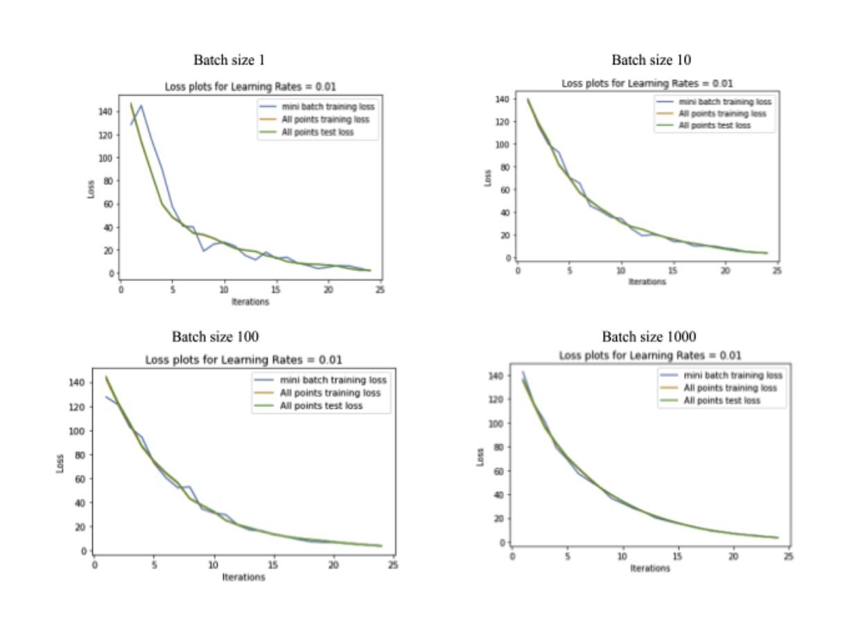
Fundamental Idea: Fundamentally, batch size dictates the amount of information our optimization algorithm can use to learn the gradient. A small batch size means there is less information at each step to update the gradient.
Effect of Convergence: With a smaller batch size the probability of the gradient jumping around is also high (as seen in our above plots as well), this would mean that convergence is slower and can take much more iterations when compared to a larger batch size.
Effect on Time/Memory: Assuming constant iterations, lr then a smaller batch size means time or memory taken is less, because then time will be = batch size * constant time taken to compute gradient. So naturally small batch size takes less time/memory but convergence (as indicated in above point) is slower.

Learning rate

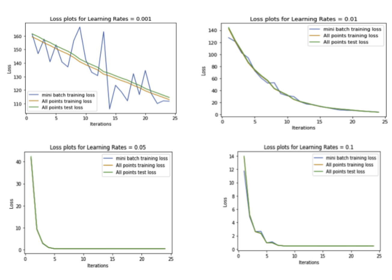
Fundamental Idea: Fundamentally, learning rate tells us how fast we move in the gradient direction. As you can see below for the batch size of 100 the convergence is not very smooth when the learning rate is too low (0.001) or high (0.1) but the it is smooth when the learning rate is in the middle (0.01, 0.05).

Share on

Twitter Facebook LinkedIn

Vaibhavi Mutya